Section 2.1 — Total Porosity
All That Empty Space
Rock might look completely solid, but up close it's full of tiny holes and spaces called pores. Porosity is simply the percentage of a rock that is empty space — the part that isn't solid mineral. Imagine a sponge: the foam is the solid part, and all the little holes are the pores. Squeeze the sponge and water comes out. Porosity tells you how much water the rock can potentially hold.
Sand and gravel have lots of pore space between the grains. Granite has almost none — it's nearly solid crystal. Sandstone falls somewhere in between, depending on how tightly the grains are cemented together. The range is enormous: from less than 1% in dense igneous rock to 45% or more in freshly deposited sand.
▶ Go deeper
Total porosity, n, is the dimensionless ratio of void volume to bulk volume: n = Vv / Vt. It is expressed as a decimal (e.g., 0.30) or percent (30%). Typical values range from ~0.01–0.05 for crystalline igneous and metamorphic rocks to 0.10–0.35 for consolidated sedimentary rocks (sandstone, limestone) and 0.25–0.50 for unconsolidated sands and gravels.
Total porosity includes all void space: connected pores, isolated pores, and pores so small that water is held by surface tension and contributes negligibly to flow. Because total porosity does not discriminate between mobile and immobile water, it overestimates the pore space available for groundwater flow and is therefore not used in contaminant transport or particle-tracking models. That role belongs to effective porosity — the subject of the next section.
Section 2.2 — Effective Porosity
Not All Holes Are Created Equal
Here's the twist: not all of those tiny holes actually help water move. Some pores are dead ends — water can sit in them but can't flow through. Others are so small that water sticks to the walls of the pore and can't be pulled out, even by a pump. Effective porosity is the fraction of pore space that actually contributes to water flowing through the rock.
Think of it like a city road network. Total porosity is every road, alley, and cul-de-sac on the map. Effective porosity counts only the through-streets — the roads that actually connect one side of the city to the other. Effective porosity is always smaller than total porosity, sometimes dramatically so.
▶ Go deeper
Effective porosity, Ne, represents the fraction of total pore volume through which advective groundwater flow actually occurs. It excludes: (1) isolated pores with no connection to the flow network, (2) pores occupied by water adsorbed onto mineral surfaces (specific retention, Sr), and (3) dead-end pore throats in which flow velocity is negligible.
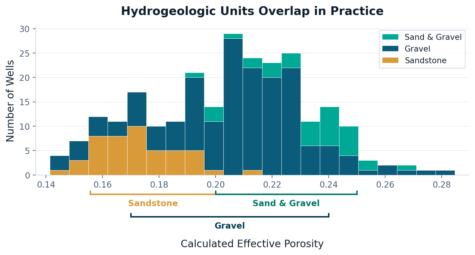
In simple unconfined granular aquifers, Ne and specific yield (Sy) are sometimes treated as approximately equal — but this comparison has important limitations that make Sy a poor substitute in practice. Specific yield is determined from aquifer pump test analysis using methods such as Theis or Cooper–Jacob, which require assumptions about aquifer geometry, boundary conditions, and test duration that are frequently not met in the field. It also varies with depth of the water table, drainage time, and the degree to which delayed yield has fully developed — meaning two analysts can derive different Sy values from the same test. In confined aquifers, karst systems, and fractured rock, Sy has no direct physical meaning at all. The Wilkinson equation sidesteps all of these issues: it requires only Q and s — two numbers measured directly in the field — and has been validated across all aquifer types with R² of 0.987–0.991. It delivers a site-specific Ne value where Sy estimation would either fail outright or require extensive additional analysis. Typical Ne values span a wide range: unconsolidated sands 0.20–0.35, sandstone 0.05–0.20, limestone 0.01–0.25 (highly variable), fractured crystalline rock 0.001–0.01.
Effective porosity is the critical parameter for computing groundwater flow velocity using Darcy's Law: v = Q / (A · Ne). It is also the cell-by-cell parameter assigned in 3D transport models such as MODFLOW/MODPATH. Assigning textbook values uniformly introduces substantial uncertainty — which is the central motivation for the Wilkinson equation.
Section 2.3 — Aquifer Types
Four Flavors of Underground Water
Not all underground water is stored the same way. The type of aquifer shapes everything: how fast water moves, how much is available, and how the rock responds when you pump. Click any panel below — a description will appear beneath the graphics.
An important fact: the Wilkinson equation has been tested across all of these aquifer types — unconfined, confined, karst, and fractured rock — with no limitations. The R² stays between 0.987 and 0.991 across every category. It doesn't matter which underground world you're working in; the equation works.
▶ Go deeper
Unconfined (Water-Table) Aquifer
Bounded above by the water table — the locus of atmospheric pressure in the saturated zone. Storage is released by gravity drainage of pore space; the storage coefficient equals specific yield (Sy), typically 0.05–0.30. Response to pumping involves delayed yield as the water table decelerates toward a new equilibrium. Rain and surface water recharge it directly from above. Where the water table intersects the land surface, a spring forms — a natural discharge point for the aquifer. Unconfined aquifers also interact directly with nearby rivers and streams: where the water table is higher than the stream stage, groundwater discharges into the channel (a gaining reach); where the stream sits higher than the water table, surface water infiltrates into the aquifer (a losing reach). Heavy pumping can reverse a gaining reach to losing, with significant consequences for streamflow.
Confined Aquifer
Fully saturated and bounded above by a low-permeability confining layer (aquitard). The hydraulic head (potentiometric surface) rises above the top of the aquifer but does not necessarily reach land surface. When it does reach land surface, the well flows without pumping — a true artesian well. Most confined aquifers are not artesian, or are only intermittently so depending on season and regional recharge conditions. Storage is released by aquifer matrix compression and water expansion; storativity is 10⁻⁵ to 10⁻³ — orders of magnitude less than unconfined aquifers. Where the potentiometric surface intersects the land surface — typically along an escarpment or valley wall — a spring can form, sometimes flowing at high rates if the aquifer is under significant pressure. Confined aquifers can also influence surface hydrology where the confining layer is thin or breached, contributing baseflow to streams and creating gaining reaches in ways that may not be obvious from surface observations alone.
Karst Aquifer
Formed in soluble rocks (primarily limestone and dolomite) by dissolution along fractures and bedding planes, producing conduit networks ranging from millimeter-scale vugs to meter-scale caves and underground rivers. Effective porosity in karst is highly heterogeneous and scale-dependent; conduit flow can be turbulent (violating Darcy's Law). The Edwards Aquifer of San Antonio, TX is a classic example.
Fractured Rock Aquifer
Occurs in crystalline or well-cemented rocks (granite, schist, quartzite, basalt) where matrix permeability is negligible and flow is controlled by fracture networks. Effective porosity is typically 0.0001–0.01. Fracture aperture, spacing, connectivity, and orientation determine hydraulic behavior. The dual-porosity concept distinguishes between high-permeability fractures (fast flow paths) and the low-permeability rock matrix (slow storage).
Page 3: The Equation →